Influence diagrams as a maintenance decision making tool

An influence diagram is a simple visual representation of a decision problem. It offers an intuitive way to identify and display the essential elements, including decisions, uncertainties, and objectives, and how they influence each other. These dependencies can be viewed more clearly than a decision tree. These diagrams, also called decision graphs, consist of a direct acyclic graph (DAG) known as its structure that depicts relationships among variables in a decision problem and conditional probabilities distribution of each node given evidence on its parents (nodes that have a direct arc into the considered node) known as its parameters. An influence diagram has 3 types of nodes as shown by the following nodes:

• chance nodes (oval shape) represent uncertain variables (environment) that influence the decision problem;

• decision nodes (rectangle shape) represent choices open to decision maker;

• value nodes (diamond shape) represent attributes (most of time numeric) the decision maker cares about.

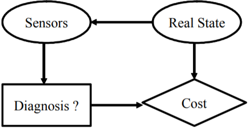
Influence diagrams are an extension of Bayesian networks that are basically DAGs consisting with chance nodes only. Bayesian Networks are driven from convergence of statistical methods that permit one to go from information (data) to knowledge (probability laws, relationship between variables, …) and Artificial Intelligence (AI), that will permit computers to deal with knowledge (not only information). The terminology comes from work by Thomas Bayes in eighteenth century. The main purpose of in these networks is to somehow integrate uncertainty in the expert system. Indeed, an expert, most of time, has only an approximative knowledge of the system that he or she formulates in terms like: A has an influence on B; if B is observed, there exists a great chance that C occurs; and so on. On the other hand, there are data (e.g. sensor measurements) that contain some information which must be transformed into relationships between variables. In influence diagrams, an arc (or edge) connecting two chance nodes is called a relevance arc because it will indicate that the value of one variable (source node) is relevant to the probability distribution of the other node (destination node), arcs from decision nodes to chance nodes are known as influence arcs. This means that the decision influences the outcome of the chance node and arcs into decision nodes (from chance nodes) are called information arcs meaning that the outcome of the chance node will be known at the time decision is made. The following figure shows an example of influence diagram that represents a decision-making problem to carry out a maintenance action. To monitor the health of the machine, some sensors are put on it in order to give information about its actual state. According to this information we can decide whether to stop the machine for maintenance or not. Stopping machine for maintenance as well as letting the machine operate in bad state has some cost. Notice that the value node representing cost node can be replaced by a chance node to represent a qualitative outcome. This mathematical tool is the backbone to construct a decision support system for decision making in uncertain and/or conflicting environment.

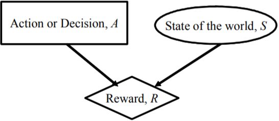
In many decision-making problems, the reward or outcome of a given decision depends on the state of the world. The principle (roughly) is as follow: there are n possible actions or decisions {a1, a2, …, an} and m possible states of the world {x1, x2, …, xm}. If an action ai is decided and the observed state of the world is xj then decision maker receives a reward r (ai, xj). This decision-making problem can be simply represented by the influence diagram:

Different algorithms are used in the literature to solve this decision-making problems, that is deciding the best action (or optimal action) knowing that the state of the world will be observed a posteriori; most popular algorithms are: Hurwicz, Savage (or MiniMax Regret) and Laplace (or Maximum Expected Value:) algorithms. These algorithms are easy to implement and computationally efficient; their main drawback is that they give an off-line (open loop) type solution. However, they do not consider a possible evidence on environmental events (absence of information link from chance node X to decision node A on the previous figure). If the state of the world were known in advance, the decision would be obvious. In most practical cases decision makers will try to estimate the state of the world by using some sensors (to be understood in large context including humans) which information is used to estimate the most probable state of the world before making decision ; this new model of decision making can be represented by the influence diagram where X is the estimation of actual state X in response to information supplied by sensors:

Application We consider a small example in the field of maintenance. The maintenance of a machine is organized in two level: for PM and CM. The PM policy consists in stopping machines periodically for a systematic maintenance process. But to avoid a possible unpredictable failure of machine, an intelligence system is implemented to continuously monitor the machines; this system consists in a number of sensors that sense some physical signals (vibration, electric signal, temperature, etc) and this information undergoes a data fusion process by a data fusion system that display the estimated status of the machine in terms of different level of warnings to the decision maker. The environment conditions (temperature, pressure, humidity, electromagnetism, …) have an influence on machine status; these conditions are not directly observed; only an estimation is available. The PM policy is established in nominal environment conditions but these conditions can be better or worst; on the basis of information displayed by data fusion system and estimated environment conditions, the reactive decision is to decide whether to ask an expert to diagnosis the machine or not. Stopping a machine in normal status for diagnosis or letting a machine fails before planned maintenance process has a cost. In terms of influence diagram, we have following nodes:

• Actual machine status (whether it is undergoing failure or not), a chance node; we suppose that this node has two states: Normal (the machine is functioning normally) and Undergoing Failure (there are troubles on the machine that could lead to its failure).

• Sensors status in terms of warnings, a chance node; the warnings correspond to machine status (green light for normal and red light for undergoing failure for instance); so, this node has two states: Green and Red.

• Environment conditions, a chance node with states Good/Bad.

• Estimated environment conditions, a chance node with states Good/Bad.

• Next status, status of machine at next observation instant, a chance node; it has two states: Failure and No Failure specifying whether the machine fails or not.

• Decision, a decision node; this node has two actions: Stop and Not_Stop.

• Cost induced, value node.

At the time decision is made, decision maker is in possession of information about sensors warnings and estimated environment conditions so there are information arcs between these chance nodes and the decision node. Sensors warnings are influenced by machine status so there is relevance arc between the later node and former one; there are also relevance arcs going from environment conditions node and machine node into future status node in one hand and from environment conditions node into estimated environment conditions node in other hand. Decision made at actual instant will influence next status of the machine so there is an influence arc from decision node to next status and finally there are functional arcs from decision node and future status node into cost node. The remaining task is to specify parameters that is start defining conditional probability distribution of each node. E.g. if sensors report right status of the machine in 95 % of cases, that is:

• Pr {SensorsWarnings = Green/ ActualStatus = Normal} = 0.95,

• Pr {SensorsWarnings = Green/ ActualStatus = Undergoing_F ailure} = 0.05,

• Pr {SensorsWarnings = Red/ ActualStatus = Undergoing_F ailure} = 0.95,

• Pr {SensorsWarnings = Red/ ActualStatus = Normal} = 0.05,