Tutorial on Principal Component Analysis

This started off as a modest attempt by me to create a tutorial on PCA… it quickly became a lot more complicated than it should have. I started asking questions to myself which I had not answers for and got confused in various places. None the less, it has helped to improve my understanding on PCA. Good luck!

What is PCA?

PCA reduces the size of data, without losing any critical information. It can be used to eliminate the redundant features in a data set, it can be used as feature selection technique, the principal components can be used as inputs for supervised learning problem and many other applications that I do not really understand. The technique basically tries to find the principal components, which are actually useful if the data is too large and understanding it is difficult. PCA will help by identifying a smaller number of uncorrelated variables that explain the maximum amount of variance.

Why we need PCA?

PCA converts original features into a new feature and the new features (transformed features space) possess the following properties:

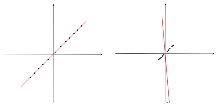
1.The correlation between new features is zero; 2.The new feature axes are called as principal component loading vectors or principal components. Our data is 2-dimensional. Therefore, two principal components can be obtained;

1. The variance of first principal component score is maximum;
2. The variance of second principal component score is second largest also the correlation between them (PC1 and PC2) is zero;

How does it work?

Suppose we have a data matrix:

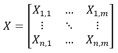
X = [n x m]

which has n samples and m measurements

you will quickly realise that if n is anything larger than 2 or 3, then just visualizing it will become e raordinarily difficult. As mentioned before, PCA can help reduce this high dimensional data into fewer dimensions. Because our suspicion is that, hopefully, not all of our data measurements are independent and there are going to be some correlations in between them.

PCA is defined as the eigen decomposition of the covariance matrix, i.e. the X(transpose).X. The dimensions of this will be a n x m matrix, and in the output, we will get a set of eigen vectors (W) and values (λ) that will describe our data. Simple?

Consider the matrix:

T = X.W

Where, the dimensions of each are:

W = [m x m] -> its columns are also called loadings

X = [n x m]

T = [n x m] -> also is called scores

Each column of W is a principal component. And because of the way this object is constructed, we will order the values in the columns of W by how large their corresponding eigen values are. So that the largest eigen is always the first one, followed by the second largest, and so on.

It should be noted that we haven’t changed our data at all but are rather describing it differently – in other words we are having the projection of all measurements in W space instead of the measurement space.

Always remember that the W matrix will have ordered columns, by the values of corresponding λs.

Now you may be wondering that I had started with X that was a [n x m] matrix and now we have T which is also an [n x m] matrix, so we haven’t really simplified anything yet. Recall that property that the eigen values in W, i.e. λ, are in order. This means that we can truncate them. We can choose to take the first R number of components and explain our data, and this ordered characteristic gives us a nice opportunity to reduce the size of the W by choosing R. e.g. we pick R = 2, then we will take the first 2 columns, or principal loadings, from our W matrix and discard everything else.

Chopping this and ignore the rest means that the dimensions on T will reduce!

This is because, once I have taken a couple of rows and got my truncated matrix, I will multiply it by X.Wr, where Wr had [m x r] dimensions:

T = [n x r]

This indicates that we can compute the principal components with a 2-dimensional representation of our data. To compute PCA there are many ways of building it, e.g., Matlab will even work with missing data and has various things to compute it.

PCA is so popular and it has been independently developed by a variety of people over the years. And in literature its goes by a lot names. I will mention only 1 over here. It turns out that doing the calculations as pointed out earlier is not the not necessarily the most computationally efficient way of computing W. Luckily there is another linear algebraic technique called Singular Value Decomposition (SVD) which is more useful. This is mathematically identical to PCA as it also does not change the relative position of any data points during operation.

Singular Value Decomposition

In SVD, X is decomposed into a product of three matrices:

X = U.σ.V*

Where * is the conjugate transpose of V

Conjugate transpose: In mathematics, the conjugate transpose of a matrix is obtained by taking the transpose and taking the complex conjugate of each element.

Let’s look at some of the nice properties of these matrices:

U is the left singular vector

V is the right singular vector

Sigma contains the singular values on its diagonal i.e. it looks like:

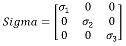
and it turns out that V is identical to W (from the PCA)

This give Sigma itself some really useful properties of the above representation:

1. These are diagonal singular values
2. They are ordered
3. U and V are unitary matrices i.e. U* U and V* V are identity matrices

Remember we had T=X.W; we now have XV = U.σ*.V

This can be simplified to

T=U.σ

From this, we can get the scores and the multiplication is much easier to do than the PCA one. And guess what, the same truncation still applies. This makes the principal component calculate using SVD super-fast!

Now the question is, how do we decide how many values we should truncate… rather how do we pick r? It is a nice property that we can truncate values but why should we choose r = 2 and not 4 or 6 from our W matrix?

It turns out that if you look at you singular/eigen values, there are a set of things that can give you the answer. We look at our σ (i.e. our singular values) and take the cumulative sum of the singular values and plot this against r. We notice that the resultant graph will settle towards a plateau, as it will approach a maximum. We then pay attention to the shape of the curve which can tell us a lot of what is happening in the system. It will tell us how much of a low dimensional our system actually is. How many numbers in the singular values we can get away with truncating.

If we get a graph which is super sharp, this means that these components can explain the whole data and there is not more variance in the data to be explained. If we get a shallow curve i.e., there is no obvious breaking point…, we have a practical problem because we can’t take all of them and choosing R becomes arbitrary. In such a case, you may want to just use r = 2 just for visualizing purposes or take a hard threshold and pick a value for r where the data is explained at around 95%.

That’s it on PCA!

Implementation

Using Matlab:

load fisheriris

X = meas;

C = (X’*X))

C =

1.0e+03 *

5.2238    2.6734    3.4838    1.1281  
2.6734    1.4304    1.6743    0.5319   
3.4838    1.6743    2.5827    0.8691   
1.1281    0.5319    0.8691    0.3023

[W, lambda] = eig(C);

W = W(:,end;-1:1)

lambda = lambda(:,end:-1:1)

%Using SVD

[U,sig,V]=svd(X);

% check now and V and W are going to be the same!

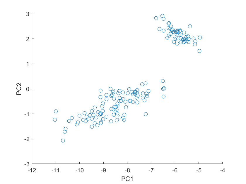
% lets project the first 2 principal components

v_r=V(:,1:2);

a=meas*v_r;

scatter(a(:,1),a(:,2))

Should we have picked r = 3 instead? we will look at the sigma values and see how much r we need; recall sigma is a 150x4 matrix

sv = diag(sig);

stairs(cumsum(sv)/sum(sv))

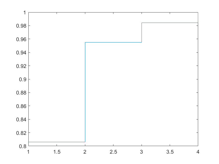
What we see is that the first singular values explain a lot of the data. We are already more than 95% by the first 2 components. This is justified by the math that simply projecting the first two columns of the v matrix will explain most of the variance in the data. You can improve visualization by using the command:

scatter(a(:,1),a(:,2),20,categorical(species))

The problem with PCA

OK I don’t know why, but for me… this is not easy to explain.

PCA is pretty good… if you have good data. If there are any anomalies or outliers though… it is too sensitive. This is not a good property and makes the route to find principal component more difficult and less fruitful.

It can breakdown with one corrupted data point or anomaly, and hence there is a need to make it more robust.

Robust PCA

RPCA is a generalization of PCA the attempts to reduce this sensitivity issue of PCAs to anomalies and outliners. It basically splits the data matrix into two parts, one which represents the low-dimensional approximation to the corrupt free data (L) and a sparsity matrix, which isolates all our corruptions (S). We need to recover these two parts:

X = L + S

X = [n x m]

Looking at above, L is unknown, its rank is unknown, S is unknown, its entries, locations, magnitudes… everything… unknown! To pursue their recovery, we need to employ a principal component pursuit:

Subject to L + S = M

Where

L

* it is the nuclear norm of the matrix; i.e. the sum of all the singular values of the matrix

S

1 is known as the L1 norm i.e. the sum of the absolute values of the entries

λ’ -> is the introduced Lagrange multiplier and is used to tune the sparsity in S

Interesting fact: The nuclear norm heuristics was introduced in 90’s, whereas the L1 norm heuristics introduced in 50’s.

We haven’t spoken much about λ’ yet. It is an important parameter and plays an important role in our calculations. A small λ’ will force more and more data to be isolated into S as being corrupt, and vice versa. If this is solely the case, then why would you ever want to choose a large value for λ’? Well there are computational resources which need to optimised after all so:

λ’ = 1/sqrt(max(n,m)).

Implementation

Implementation using PCP is straight forward using alternating directions. The alternating direction method of multipliers (ADMM) is an algorithm that solves problems by breaking them into smaller pieces, each of which are then easier to handle. It is a variant of the augmented Lagrangian scheme that uses partial updates for the dual variables, in our case, L and S.

initialize: S0, Y0 and τ > 0

while not converged

Lk = Dτ (M − Sk−1 + Yk−1) (shrink singular values)

Sk = Sλτ (M − Lk + Yk−1) (shrink scalar entries)

Yk = Yk−1 + (M − Lk − Sk)

end while

output: L, S

Dτ and Sλτ are shrinkage operators for singular values and scalar entries respectively.

Download the Matlab script for RPCA from here.

When we run the above algorithm on the fisheriris data, we are able to pick up some corruptions/anomalies in the data. Below is sparsity matrix plot:

Of course, this was just to demonstrate the fact that the algorithm works. We can separate L and S.